最近的
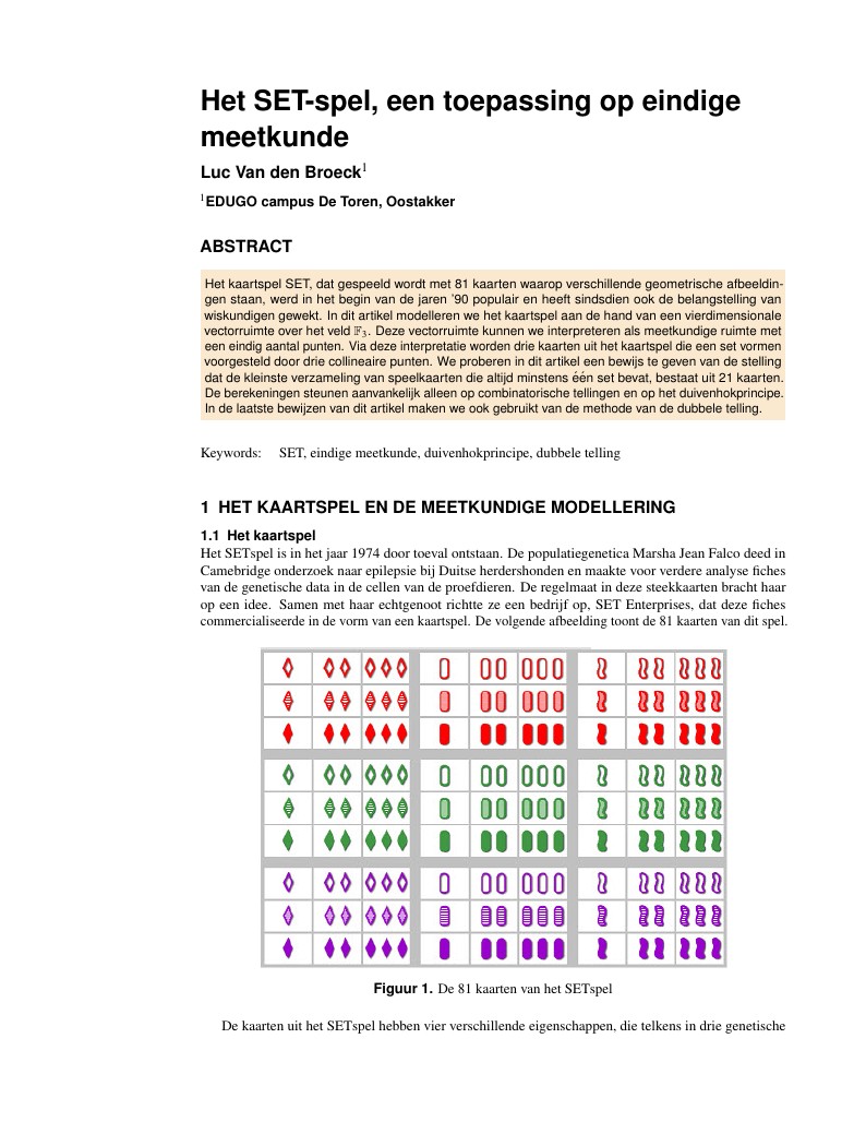
Het kaartspel SET, dat gespeeld wordt met 81 kaarten waarop verschillende geometrische afbeeldingen staan, werd in het begin van de jaren '90 populair en heeft sindsdien ook de belangstelling van wiskundigen gewekt. In dit artikel modelleren we het kaartspel aan de hand van een vierdimensionale vectorruimte over het veld 𝔽3. Deze vectorruimte kunnen we interpreteren als meetkundige ruimte met een eindig aantal punten. Via deze interpretatie worden drie kaarten uit het kaartspel die een set vormen voorgesteld door drie collineaire punten. We proberen in dit artikel een bewijs te geven van de stelling dat de kleinste verzameling van speelkaarten die altijd minstens één set bevat, bestaat uit 21 kaarten. De berekeningen steunen aanvankelijk alleen op combinatorische tellingen en op het duivenhokprincipe. In de laatste bewijzen van dit artikel maken we ook gebruikt van de methode van de dubbele telling.

Principal Components Analysis (PCA) and Canonical Correlation Analysis (CCA) are among the methods used in Multivariate Data Analysis. PCA is concerned with explaining the variance-covariance structure of a set of variables through a few linear combinations of these variables. Its general objectives are data reduction and interpretation. CCA seeks to identify and quantify the associations between two sets of variables i.e Pulp fibres and Paper variables.PCA shows that the first PC already exceeds 90% of the total variability. According to the proportion of variability explained by each canonical variable , the results suggest that the first two canonical correlations seem to be sufficient to explain the structure between Pulp and Paper characteristics with 98.86%. Despite the fact that the first the two canonical variables keep 98% of common variability, 78% was kept in the pulp fiber set and about 94% of the paper set as a whole. In the proportion of opposite canonical variable,there were approximately 64% for the paper set of variables and 78% for the pulp fiber set of variables kept for the two respectively.

A lecture on intermediate proofs that I taught at ARML.
Linear regression is one of the most widely used statistical methods available today. It is used by data analysts and students in almost every discipline. However, for the standard ordinary least squares method, there are several strong assumptions made about data that is often not true in real world data sets. This can cause numerous problems in the least squares model. One of the most common issues is a model overfitting the data. Ridge Regression and LASSO are two methods used to create a better and more accurate model. I will discuss how overfitting arises in least squares models and the reasoning for using Ridge Regression and LASSO include analysis of real world example data and compare these methods with OLS and each other to further infer the benefits and drawbacks of each method.
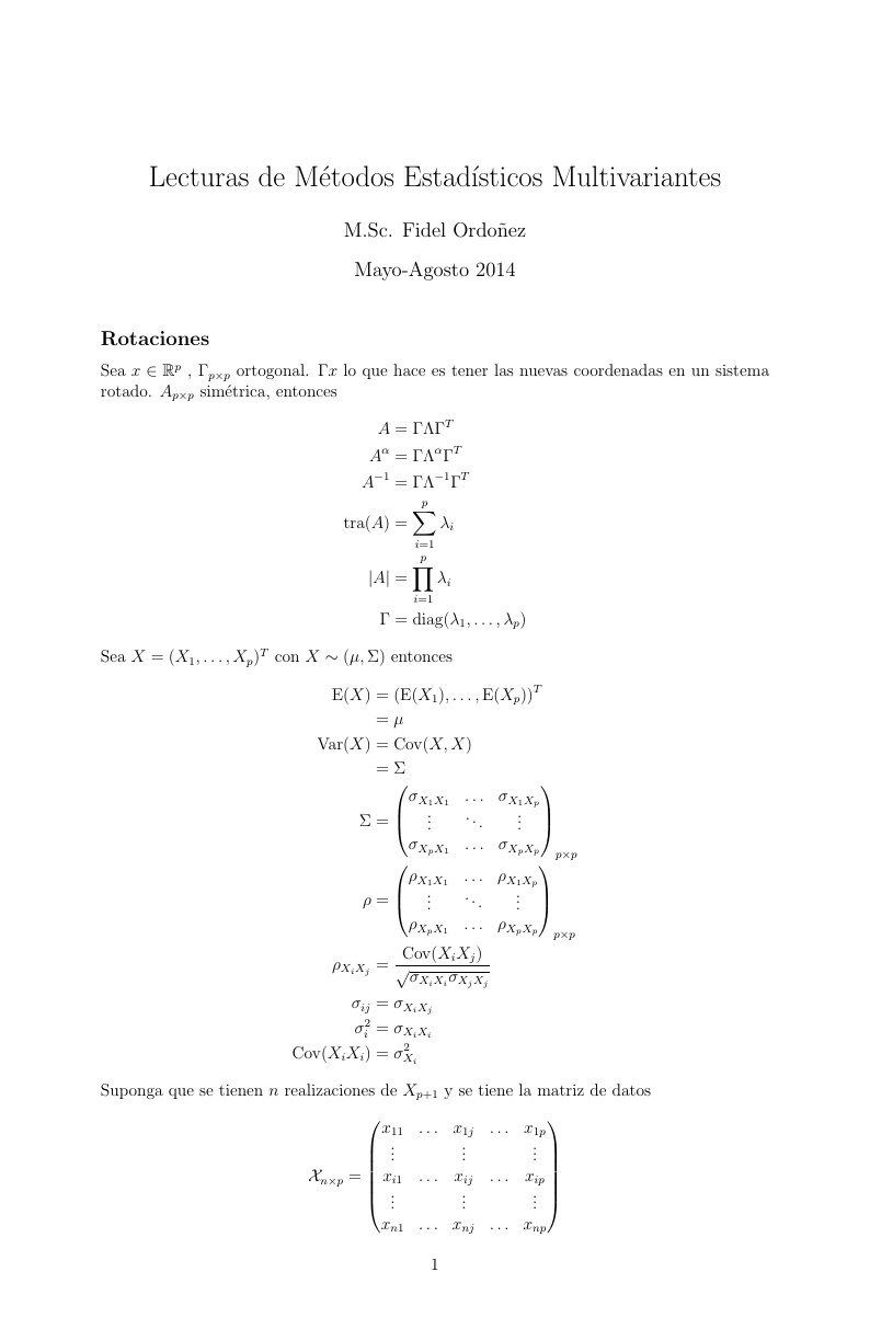
Lecturas tomadas de la clase de M.Sc. Fidel Ordoñez, Carrera de Matemática UNAH, 2014
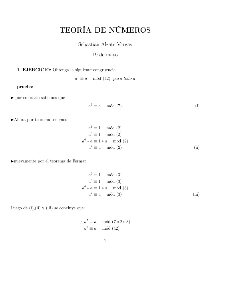
Teoría de números
The objective is to study the effect of different experimental parameters on the reconstruction of the density of states (DoS) and to verify the viability of the 1D/2D simulation model developed at GeePs. Beside the calculation of the DoS through the modulated photo-current method (MPC), the ambipolar minority carrier diffusion length is measured through steady state photocarrier grating (SSPG) and the majority carrier lifetime / mobility product is measured through steady state photo-conductivity (SSPC). The measurements were observed to be in agreement with the theoretical simulations, but further experiments are needed to accurately conclude the need of a 2D simulation for the MPC experiment.
In this note, we will show how transformations can be used to obtain a radically simple derivation of the equation of the line of best fit. Our approach also gives a simple geometric interpretation of the Pearson correlation coefficient.
In this paper, we derive and prove, by means of Binomial theorem and Faulhaber's formula, the following identity between $m$-order polynomials in \(T\) \(\sum_{k=1}^{\ell}\sum_{j=0}^m A_{m,j}k^j(T-k)^j=\sum_{k=0}^{m}(-1)^{m-k}U_m(\ell,k)\cdot T^k=T^{2m+1}, \ \ell=T\in\mathbb{N}.\)